Collision Avoidance Algorithm: VO vs RVO vs ORCA (RVO2)
Background
In the vast and intricate world of game design and development, characters are often guided by sophisticated path-finding algorithms, such as the renowned A*, to navigate through the complex landscapes of the game map. These algorithms serve as the characters’ compass, leading them through the labyrinth of the virtual world, from their current location to their intended destination.
However, the journey is not as straightforward as it seems. The A* algorithm, while efficient in charting a course, does not account for the dynamic nature of the game environment. It doesn’t consider the specific states of all navigating individuals or the motion states of other agents in the vicinity. Instead, it perceives all objects as obstacles, which complicates the map and significantly increases the path planning time.
Imagine yourself as a DoorDash driver, navigating through the bustling city streets. Your route from your current location to the delivery destination is primarily determined by a high-level path planning algorithm, similar to A*. This algorithm ensures the shortest path from your starting point to your goal. However, just like in the gaming world, this high-level path planning doesn’t account for the real-time dynamics of the city traffic.
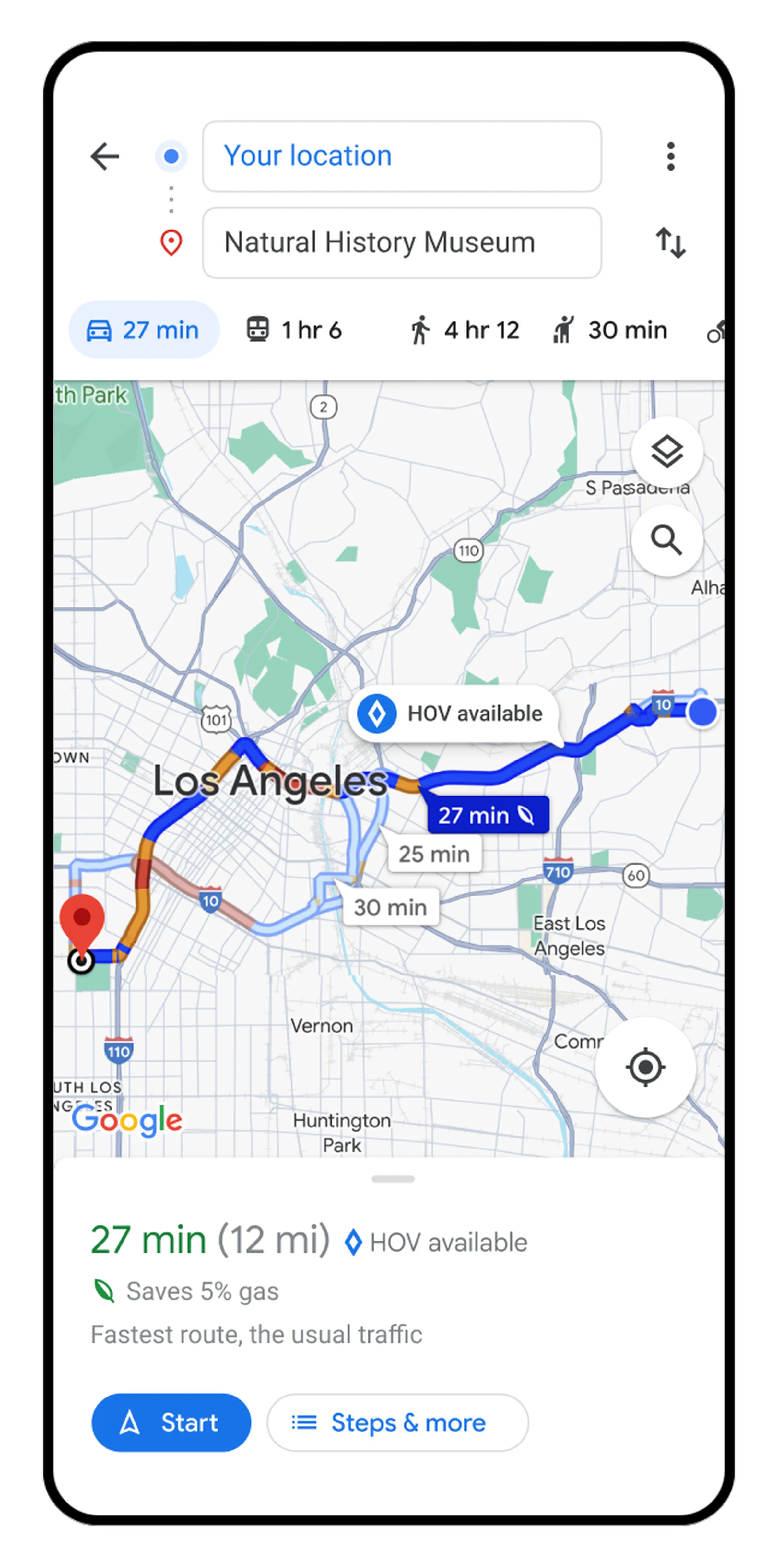
While on the road, you may encounter other vehicles and buildings. Navigating around these obstacles involves the use of collision avoidance algorithms. It’s important to note that, even while avoiding collisions, the driver should not deviate significantly from the planned route. In other words, no matter how much you need to dodge other vehicles, you should still remain approximately on the established route.
For collision avoidance algorithms, velocity obstacle (VO)-based algorithms are more commonly used in game development nowadays, because its computation is distributed and the process is simple, which is very suitable for large-scale unit collision avoidance scenarios. Currently its algorithm has been optimized to ORCA, but before that, it is better to start with VO, so that it is easier to understand the gradual optimization evolution of the algorithm.
All three algorithms (VO, RVO, ORCA) are used more for a local navigation, it can only perceive the situation close to its own surroundings, without the information of the global environment, and it only manages to navigate without colliding with the surrounding individual goals or obstacles. At this point, there is a complementary relationship with the traditional path-finding algorithm A*.
So in this article, we will describe the algorithms in the most vernacular way possible (e.g., for Minkowski Sums, etc., we will represent them all geometrically).
Velocity Obstacle (VO)
VO is not really an algorithm, it’s just a way to solve the collision avoidance problem, and the subsequent RVO and ORCA are all based on this setup.
It puts forward a kind of thing called Velocity Obstacle, in fact, it is also very intuitive to know the meaning. It is equivalent to a series of possible collision velocity in the velocity domain (geometric space is expressed as a horizontal and vertical velocity-based coordinate system) as a need to avoid the region, in the choice of the speed of the next frame, to avoid the speed of the region on the good.
Concept
Supposes a scenario, A and B meet in space, because the VO algorithm itself is distributed, that is, each object only consider the object itself. We consider the encounter from the point of view of A.
We assume that A and B have their own social safety distance, this distance is a circular range, the radius is $R_a$ and $R_b$. Then, naturally think of the algorithm as our relative movement of this frame to ensure that the closest distance between the two agents to be greater than or equal to $R_a + R_b$.

Thus, it is obvious the way to achieve this goal is very simple: place a mass point at agent A‘s position, and then place a large circle with radius $R_a + R_b$ at agent B‘s position. All the positions outside the circle are relatively safe for A go to. So, the relative movement of the frame can be outside the circle as long as it lies outside the circle.
Although the ending position can be outside the circle, the path we move is actually a straight line from the initial A‘s position to its ending position.
Because the moving process is continuous, so we also need to make sure that we don’t “pass through” the great circle to reach the back of the gray circle, that is, the conical region behind the gray circle with respect to the position of the mass point is also unreachable.
It is fairly obvious as we are drawing a geometric figure:

As shown above, the gray area is the unreachable area, but for simplicity of computation and some predictive effect, the VO algorithm treats the entire triangular area as a dangerous area.
At this time, the relative displacement of the said frame of the mass, in fact, is the single-frame velocity of the mass point. And the single-frame velocity of the mass, in fact, is the relative velocity of A and B. So, in fact, we can very easily map the above figure to the velocity domain, the origin of its coordinate system being the coordinates of the agent A, the mass point.
You can see that the graph below, the geometric structure is basically the same as the above diagram, except that this has been mapped to the velocity domain (red area in the coordinate domain is the danger zone, in the velocity domain that is the VO).

Theoretically, A and B can be safely staggered when their relative velocities choose a point outside the red triangle.
Relative Velocity Obstacle (RVO)
The idea of VO is very simple, but the flaw is also very obvious, that is, jitter can occur, and possibly happens even in the case of only two agents, let’s look at the original example.

When A and B are traveling in opposite directions, initially A and B will stagger. But when the speed of the other changes in the next frame, they will turn their speeds back, because at this point, A will think that B is just going up to the left, so I won’t collide if I still keep my optimal downward motion, and B will think the same, so they turn back.
In fact, this probably won’t result in an eventual collision either, because in the second frame their speeds are indeed staggered, so they’ll still end up dangerously staggered due to the predicted collision.
However, the process of repeated horizontal jumps of the two agents in this process is still not elegant enough, and the reason for this is obvious; the VO algorithm has agents that always default to the other agents being stable and moving at a constant speed, which leads to their own behaviors becoming out of line with expectations when the other’s speed changes.
So the biggest improvement in RVO is that we assume that the other side will also use the same strategy as us, instead of maintaining a constant speed .
Concept
In the basic VO algorithm, the reason for the jitter is that after A chooses a new speed in frame 2, he realizes that B‘s speed has also changed a lot, and A thinks that changing back to the optimal speed (i.e., the one that points directly to the destination) does not seem to be a collision either, because B‘s new speed is actually changed under the assumption that A can keep the optimal speed without collision, so A thinks that B allows him to turn back, but at the same time B also thinks the same thing.
However, in the RVO algorithm, A only changes his speed by $\frac{1}{2}$, that is, if A and B want to be staggered, they need to be staggered by a total of 10cm. In the VO algorithm, both A and B will each be staggered by 10cm, while in the RVO algorithm, A will only be staggered by half, that is, 5cm, and at the same time A assumes that B will be staggered by the other half, which is what B thinks as well. Therefore, by coincidence, the second frame, each person is staggered by half, and found that at this time to turn back to the optimal speed is still a collision (because each person makes only half of the turn), so effectively avoid the phenomenon of the above jitter.
Optimal Reciprocal Collision Avoidance (ORCA/RVO2)
While RVO solves the problems that arise with the VO algorithm and almost always performs well in one-to-one obstacle avoidance, it still fails to meet expectations when the number of agents increases.
Assuming the following scenario, where A and B are traveling in a left and right side of C, what happens in RVO?

A thinks that C will turn right, so he turns $\frac{1}{2}$ left, and B thinks that C will turn left, so he turns $\frac{1}{2}$ right, and C actually has no choice either way, because in the VO diagram, it’s actually two cones in front of him, so C chooses to try very hard to turn left or right.
At this point, A, B, and C are all screwed up 👿, because none of their predictions are correct, so they modify their own speed at frame 3 based on an unanticipated opponent’s speed, thus creating jitters again.
The reason for this is actually quite simple: in RVO, all the agents assume that the other is only thinking about itself.
So the cause of this accident is that A thinks C loves him, and B thinks C 😍 him, but in reality C 😍 both of them at the same time, as if A was looking for C to go on a date, and then C brought B along.
Although there’s no real collision in this case, because A and B will eventually move to the left and right, and jitter in the process is not what you’d expect.
And this is how ORCA came from, which actually solved this jitter problem (although I think it came out by chance, since the improvement of ORCA over RVO was mainly due to efficiency).
The biggest difference between ORCA and RVO lies in the shape of the VO. In previous VO algorithms, the VO appears as a cone of infinite height, which in 2D is the angle between two rays of the same origin, but in ORCA, we use a directed plane to divide the space.
Thus, the computation to solve for the optimal speed is also optimized, from a space cut by a bunch of sharp corners to a linear programming problem.
Concept
And how does ORCA get this plane? Let’s look at the diagram.

First we still have to understand the diagram, $p$ is the position of the two points, $r$ is the radius of the two agents, and $\tau$ is the unit time (I don’t know why he used the letter $\tau$, maybe because it’s the etymology of $t$?).
Fig. a) is the positional domain, where agents A and B meet by chance.
At this time, we look at the problem from the perspective of A. Putting the position of A to the origin, the position of the unreachable region of the VO algorithm in the position domain is the same as the part of the large circle in Fig. b) and the conical space behind it, i.e., the circle with $p_B-p_A$ as the center and a radius of $r_A + r_b$.
In the velocity domain, the distance traveled per unit time $t$ (i.e., the set frame interval, and also the warning time to start obstacle avoidance) can actually be interpreted as the velocity, so it is guaranteed that after $\tau$ time, it will not enter the $VO$ region at the above location, i.e., the gray region in Fig. b).
This is not difficult to understand, right? You use the speed on the small circle, just after $\tau$ time will be to the position of the large circle, so the $VO$ as in Fig. b).
In Fig. c), we do not care about it, in fact, is to facilitate our understanding, but I think in fact, it does not help us understand ORCA at the moment.
If the $VO$ here is interpreted as a cone, it is still similar to the previous VO, but ORCA is interpreted as a biplane, the plane is about the following figure:

That’s the plane that the red arrow is pointing to. Don’t worry about the mosaic, that’s the plane of agent B. We’re in agent A, so we can’t see it.
First I’ll explain the variables in the diagram. $V^{opt}$ refers to the desired velocity of the two agents, which is generally the velocity pointing to the destination, $u$ is the shortest vector from $V_A^{opt}-V_B^{opt}$ to the boundary of the $VO$ region, and $n$ is the outward normal of the boundary of $VO$ at point $\left(V_A^{opt}-V_B^{opt}\right)+u$.
At this point, the plane is determined, which is the half-plane pointing in the direction of $n$ starting at the point of $V_A^{opt}$ + $u/2$.
Why is it determined this way? I believe that some of you already know. $u$ is what, $u$ is in fact the value of the relative velocity that needs to be modified, equivalent to the example of 10cm above. So, $V^{opt} + u/2$ is in fact equivalent to the best modified speed in the dispute between A and B. Up till this poin it is almost the same as the RVO.
The difference is that we don’t use this value as part of the final answer when we get it, but rather we determine the half plane from it.
With this, first we have to explain why we want to determine a half-plane? As I said before, the use of the half-plane can be transformed into a simple linear programming problem, the amount of computation plunge off a cliff.
So why do we choose this half-plane besides the computation efficiency? The actual reason is actually very simple, this is the half-plane that contains the best solution to this current conflict.
Therefore, when A in the completion of a number of planes of cutting, each plane cuts the remaining optional half-plane, must contain the best solution to the current conflict speed. For example, the speed with B must be contained in the first half-plane, and the best speed with C must be contained in the second half-plane!
This ensures that within the intersection of so many half-planes, the likelihood of an optimal speed with each opponent's solution is maximized, and even if the optimal speed ends up being cut away, a relatively better speed can always be chosen.
Personally, I think this conclusion the easiest way to understand, so I won’t go into the proof here, as it defeats the purpose of talking about the algorithm in broad terms.
Special Case
Ok then after the space is cut, if the optimal velocity is in the current plane, the optimal velocity is chosen. Otherwise, the closest velocity to the optimal velocity in the post cut plane is chosen, which is generally located at the boundary vertices of the plane, and translates into a simple linear programming problem.

This is the figure in the paper, note that there is a curve in Fig. b). This is because there is also a $V_{max}$ in the paper, i.e., the maximum speed that the agent can reach, which is reasonable, but it is not part of the core of the algorithm, so I didn’t talk about it earlier.
Of course, it should be noted that when there are a lot of agents, it is very easy for ORCA to cut out the entire space, because as I said before, it cuts out almost half of the space every time, so it is very easy for this to happen.
The solution to this situation is actually very simple, is to add a variable d, which represents the distance of the velocity to the current half-plane, d is positive means that the current velocity is within the half-plane, negative means that the half-plane is cut off, we are looking for the maximum sum of d corresponding to the speed, which is also equivalent to the smallest velocity of the violation.
Geometrically, it is much more intuitive, how to understand it is to move the half-plane outward, so that the half-plane has less cut parts, so that these half-planes just cut out a point, at the same time, the least translation of all the half-planes, choose this point as the target speed.
Static Obstacles Avoidance
In addition, the paper also discusses about static obstacle avoidance, in fact, it is reasonable, because you can not just avoid moving things when you deliver food, but also to avoid light poles.
The logic of this is actually very simple, that is, because the obstacle itself does not have velocity, so an agent body has all the responsibility for avoidance, rather than $\frac{1}{2}$.
The complexity of the code is mainly because the obstacle is not a moving circle, but a line segment connected to a polygon, so the calculation is much more complex.